


BISAC NAT010000 Ecology
BISAC NAT045050 Ecosystems & Habitats / Coastal Regions & Shorelines
BISAC NAT025000 Ecosystems & Habitats / Oceans & Seas
BISAC NAT045030 Ecosystems & Habitats / Polar Regions
BISAC SCI081000 Earth Sciences / Hydrology
BISAC SCI092000 Global Warming & Climate Change
BISAC SCI020000 Life Sciences / Ecology
BISAC SCI039000 Life Sciences / Marine Biology
BISAC SOC053000 Regional Studies
BISAC TEC060000 Marine & Naval
Polar lows are generally characterized by severe weather in the form of strong winds, showers and occasionally heavy snow, which have sometimes resulted in the loss of life, especially at sea. Numerical simulations with mesoscale atmospheric models is a good alternative to investigate polar low phenomenon, because they produce temporally and spatially regular-spaced fields of atmospheric variables with high resolution. To describe the evolution of atmospheric processes the Advanced Weather Research and Forecasting (WRF-ARW) model was used. The principal objectives of this study were 1) the understanding of mesoscale WRF model and adapting the model for the Barents Sea region; 2) to conduct numerical experiments using WRF model with different Planetary Boundary Layer parameterization (PBLs) schemes and investigate the impact of each scheme on the quality of forecast; and 3) the investigation of the capability of WRF model to successfully simulate evolution of polar lows. The impact on the quality of forecast was investigated. The results of the study, obtained by numerical modeling of polar mesoscale low over the Barents Sea. One polar low, near Spitsbergen, from 24 of March to 26 of March 2014 were targeted. The results of numerical experiments showed that each of Planetary Boundary Layer parameterization scheme isn't successful for simulation of polar low.
WRF-ARW, polar low, Planetary Boundary Layer parameterization (PBLs) schemes
I. INTRODUCTION
Arctic atmosphere unique natural event - polar mesoscale cyclone. These synoptic systems were discovered and documented in the middle of ХХ century based on atmosphere satellite sounding methods development. Polar lows are intense mesoscale cyclones that are associated with cold air outbreaks and form poleward of the main baroclinic zone. Sometimes referred to as Arctic hurricanes, polar lows are short-lived (less than 48 h) and small-scale (less than 1000 km) cyclones, unlike their tropical counterparts. What they do have in common is strong surface winds: at least gale force is required for a polar low. These definition and set of criteria became
conventional since their publication by Rasmussen and Turner [1] and are used throughout this letter. Polar mesocyclones capture an intensive attention of sea transport staff, meteorologists, oceanologists, climatologists and Arctic shelf oil extraction specialists. This information is usefull to support the Hydrometeorological service and to increase the quality of forecasting over Arctic sea area of water where mesoscale cyclogenesis processes develop. Unfortunately, we have no data, which have enough spatial and temporal resolution, for provide complete set of meteorological variables, needed for thorough study of their dynamics, underlying physical mechanisms and factors for forming polar lows. Therefore, numerical simulations with mesoscale atmospheric models is a good alternative to investigate polar low phenomenon, because they produce temporally and spatially regular-spaced fields of atmospheric variables with high resolution.
In this study, the planetary boundary layer (PBL) depicted in high resolution Weather Research and Forecast Model (WRF) simulations of polar low over Barents Sea in 2014 is studied and evaluated by direct comparisons with satellite data. In particular, two boundary layer schemes are evaluated: the Yonsei University (YSU) parameterization and the Mellor-Yamada Janjic (MYJ) parameterization. Investigation of these schemes is useful since they are available for use with WRF, are both widely used, are based on entirely different methods for simulating the PBL, and results of this study will be used in assimilation satellite data for simulation of polar lows.
To describe the evolution of polar low atmospheric processes , the Weather Research and Forecasting model of Advanced Weather Research core (WRF-ARW) version 3.1 has been used.
To achieve this goal, the following principal tasks were involved:
- The understanding of mesoscale numerical WRF model and adapting the model over;
- To conduct numerical experiments using WRF model with different Planetary Boundary Layer (PBL) parameterization schemes and investigate the impact of each scheme on the quality of forecast;
- The investigation of the ability of mesoscale numerical WRF model to successfully simulate evolution.
The task of using mesoscale WRF model for the purpose of improving the quality of evolution polar low forecast is very important. WRF model is a numerical weather prediction (NWP) and atmospheric simulation system designed for both research and operational applications. WRF is supported as a common tool for the research and operational communities to promote closer ties between them and to address the needs of both. The development of WRF has been a multiagency effort to build a next-generation mesoscale forecast model and data assimilation system to advance the understanding and prediction of mesoscale weather and accelerate the transfer of research advances into operations. WRF-ARW is a fully compressible non-hydrostatic model which use time splitting scheme in order to increase model efficiency. The equations used in the model allow acoustic waves due to their compressibility nature and therefore require short time step for the model stability to be achieved. Slow waves which are of meteorological important are integrated using a third-order Runge-Kutta (RK3) time integration scheme, while the high-frequency acoustic modes are integrated over smaller time steps to maintain numerical stability. For spatial discretization WRF-ARW model uses Arakawa C grid staggering due to the fact that it conserve mass and energy for long run simulations. Advantage of using WRF model is that it provides a large set of options from which to choose suitable parameterization scheme for the description of physics of non-adiabatic processes[2].
II. STUDY AREA
Barents Sea is region where polar lows frequently form. Significant thermal contrasts in the surface layer, which forced by proximity the drifting ice, and the penetration of warm Atlantic waters to the north, combined with the intense tropospheric transference create conditions for the development of baroclinic instability in the region during the cold season. The main sources of energy in the formation and development of polar mesocyclones are turbulent fluxes of heat and moisture from the sea surface.
Study of this region is interested by rapid development of oil and gas.The Barents Sea is great importance for the transport and fishing - there are large ports, oil and gas platforms. All of these have great importance for Russia.
III. DATA AND METHODOLOGY
To describe the evolution of polar low over Barents Sea, the Weather Research and Forecasting model of Advanced Weather Research core (WRF-ARW) Version 3.6.1 has been used. WRF is a nonhydrostatic, fully compressible mesoscale model of atmospheric dynamics [3].
The outermost domain for all simulations has 120x120 grid points with 10 km grid spacing in the zonal (x) and meridional (y) directions. The domain is centered at latitude 77.0 N and longitude 35.0W. WRF uses map factors to account for the curvature of the Earth, which for this case were computed using a North Polar Stereographic map projection.
In the vertical direction, 35 half and correlative 34 full  -levels are applied. As polar lows are shallow weather phenomena, which are highly influenced by physical processes in the boundary layer, user defined η-levels are specified in this thesis to increase the vertical grid resolution near the surface.
Initial and boundary conditions for these simulations are computed from the initial conditions (reanalysis) NCEP/NCAR[4]. Initial conditions must specify the three-dimensional distribution of three velocity components, temperature, pressure and humidity, and the boundary conditions for temperature, humidity and velocity components, as well as the heat, moisture and momentum fluxes at the lower boundary of the model domain.
IV. RESULTS
For WRF model adaptation for modeling atmospheric processes over Barents Sea, numerical experiments were conducted. Simulations were conducted for 48 hours from 00 UTC 24 of March 2014.
.jpg)
We focus on the evaluation and comparison of two particular PBL schemes: the Yonsei University scheme [5] and the Mellor-Yamada-Janjic scheme [6]. These two schemes are available in standard versions of the Weather Research and Forecast (WRF) model that is now used widely for both operational weather forecasts and research [3] . There are other very good reasons for considering them. First, they are based on fundamentally different approaches to simulating the PBL; and second, even outside of the WRF model, these two parameterizations, or close cousins to each, are both used widely in hurricane simulations and forecasting.
The Mellor-Yamada-Janjic (MYJ) scheme is an updated and modified version of the original Mellor-Yamada boundary layer parameterization [6] implemented for use in numerical weather prediction by Janjic [7]. The MYJ scheme is commonly referred to as a “level 2.5” model, based on the 4 “levels” of complexity for PBL schemes originally proposed by Mellor and Yamada [6]. The level 2.5 scheme was introduced later as intermediate to levels 2 and 3. The MYJ scheme predicts the generation, vertical transport, diffusion, advection, and dissipation of turbulent kinetic energy (TKE). It should be noted that in the WRF version of the MYJ scheme, TKE is not advected horizontally. This is in the spirit of the “lubrication approximation”: since vertical gradients of all quantities are much greater than horizontal gradients, horizontal advection terms are expected to be small. The TKE, local gradients, and a diagnosed length scale are used to compute spatially varying eddy viscosities for momentum, heat, and moisture, which are then used to compute turbulent diffusion of these substances in the boundary layer. The surface layer is actually divided into two layers, with a traditional Monin-Obukhov surface layer adjacent to the surface, and a level 2 type MellorYamada model (with diagnosed TKE) in between the lower surface layer and the 2.5 level scheme above. The MYJ scheme is considered a “local” scheme because the tendencies at each location depend only on the properties of the flow and the value of the TKE at and immediately nearby that location [8].
To summarize, the MYJ PBL scheme predicts the generation and redistribution of TKE in the boundary layer, uses the value of TKE to compute a spatially varying eddy viscosity, and then diffuses simulated quantities vertically in the boundary layer.
The Yonsei University scheme [5] is an updated and improved version of the scheme previously known as the “MRF” scheme, based on its use in the medium range forecast model at the National Centers for Environmental Prediction [9]. In turn, the MRF scheme was based on prior development of a simplified, non-local boundary layer parameterization by Troen and Mahrt . Here, the term “non-local” refers to the fact that the PBL tendencies at each location are ultimately related to the flow and temperature profiles throughout the depth of the boundary layer. More specifically, the depth of the boundary layer is first estimated as the height where the potential temperature matches the virtual potential temperature of a parcel at the surface: that is, the expected height at which parcels from the surface can rise through a well-mixed layer. A profile of eddy viscosity that increases linearly from the surface, reaches a peak value in the middle of the boundary layer, and then decreases to near zero at the top of the boundary layer, is then matched to fit within the diagnosed boundary layer height. The PBL tendency is the divergence of this diffusive flux plus two additional fluxes: vertical fluxes of momentum, heat, and moisture are also incorporated to account for transport by large eddies, and additional vertical fluxes are added to account for entrainment at the top of the boundary layer. Fluxes at the surface are computed through the usual Monin-Obukhov theory with bulk exchange coefficients.
To summarize, in the YSU PBL scheme, the depth of the well-mixed layer is estimated, a profile of eddy-viscosity is prescribed to fit within this layer, and additional fluxes are added to account for large-eddy transport and boundary layer top entrainment.
Fixing the mixed layer model parameters to their control values, we compare track and pressure of polar mesocyclone with the two different PBL schemes, as shown in Fig.2.
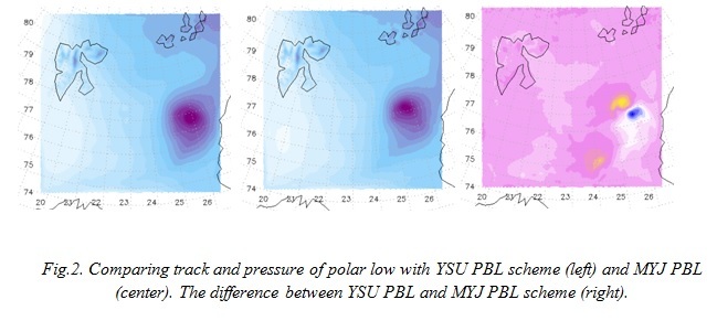
The polar low center is determined with small differences, yellow shows difference (at 3 hPa) in location of center at the right picture. To compare modeled fields with fact, we used satellite data. It shown that first parametrization is better. The center of mesocyclone and pressure at that point are matched.
Figure 3 shows water vapor field of YSU PBL scheme and MYJ PBL scheme, also observational data from MODIS (Moderate Resolution Imaging Spectroradiometer)[11].
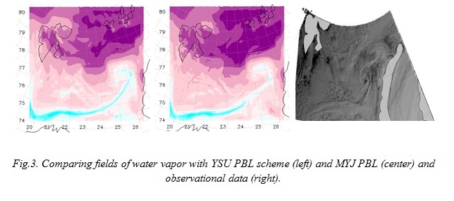
Comparing the cloud structure (satellite image) with water vapor fields, it can be said that the Yonsei University scheme is clearer. To determine the center of low and rains, it is important.
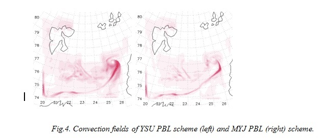
To analysis, convection we used index CAPE (Convective Available Potential Energy) is one of the latest weather indices that measure atmospheric instability. Therefore, CAPE indicates parcel buoyancy highlighting how rapidly an air parcel will rise in the atmosphere. Rising air then cools and condenses forming clouds and thunderstorms. We see the Yonsei University scheme (left) gives more interesting and informative field. In this case, we can’t compare modeled fields with satellite data, and to determine the best, we choose which shows the mesocyclone area more clearly.
V. CONCLUSION
For the mesoscale WRF model adaption for modeling of atmospheric process over Barents Sea, numerical experiments were conducted. Evolution of polar low was carried out for 48 hours starting from 00Z from 24th to 26th March 2014.
All the simulations with varying PBL schemes and varying horizontal and vertical resolutions produced very similar tracks. But the Yonsei University scheme is better scheme for simulation polar mesocyclones.
Results of this study will be considered at next step of polar low research. We are going to simulate polar lows with assimilation satellite data.
1. Rasmussen, E. A. and J. Turner, 2003: Polar Lows: Mesoscale Weather Systems in the Polar Regions. Cambridge University Press, 612 pp.
2. Mlawer, E. J., S. J. Taubman, P. D. Brown, M. J. Iacono, and S. A. Clough, 1997: Radiative transfer for inhomogeneous atmosphere: RRTM, a validated correlated-k model for the longwave. J. Geophys. Res., 102(D14) 16663-16682.
3. Skamarock, W. C., J. B. Klemp, J. Dudhia, D. O. Gill, D. M. Barker, W. Wang, and J. G. Powers, 2005: A Description of the Advanced Research WRF Version 2. NCAR technical note 468+STR, 88 pp.
4. Kanamitsu, M., et al. (2002a), NCEP dynamical seasonal forecast system 2000, Bull. Am. Meteorol. Soc., 83, 1019 - 1037, doihttps://doi.org/10.1175/1520- 0477(2002)0832.3.CO;2.
5. Noh, Y., W. G. Cheon, S. Y. Hong, and S. Raasch, 2003: Improvement of the K-profile model for the planetary boundary layer based on large eddy simulation data. Bound.-Layer Meteor., 107, 421-427
6. Mellor, G. L., and T. Yamada, 1982: Development of a turbulence closure model for geophysical fluid problems. Rev. Geophys. and Space Phys., 20, 851-875.
7. Janjic, Z. I., 1990: The step-mountain cordinate: Physical package. Mon. Wea. Rev., 118, 1429- 1443.
8. Nolan, D. S., D. P. Stern, and J. A. Zhang (2009b), Evaluation of planetary boundary layer parameterizations in tropical cyclones by comparison of in situ observations and high-resolution simulations of Hurricane Isabel (2003), Part II: Inner-core boundary layer and eyewall structure, Mon. Weather Rev., 137(11), 3675-3698, doihttps://doi.org/10.1175/2009MWR2786.1.
9. Hong, S.-Y., and H. L. Pan, 1996: Non-local boundary layer diffusion in a medium-range forecast model. Mon. Wea. Rev., 124, 2322-2339.
10. Troen, I., and L. Mahrt, 1986: A simple model of the atmospheric boundary layer: Sensitivity to surface evaporation. Boundary-Layer Meteorol., 37, 129-148.
11. Smirnova J.E., P.A. Golubkin, L.P. Bobylev, E.V. Zabolotskikh, B. Chapron, (2015). Polar low climatology over the Nordic and Barents seas based on satellite passive microwave data . Geophysical Research Letters, doihttps://doi.org/10.1002/2015GL063865 IF 4.196.