


Russian Federation
BISAC NAT010000 Ecology
BISAC NAT045050 Ecosystems & Habitats / Coastal Regions & Shorelines
BISAC NAT025000 Ecosystems & Habitats / Oceans & Seas
BISAC NAT045030 Ecosystems & Habitats / Polar Regions
BISAC SCI081000 Earth Sciences / Hydrology
BISAC SCI092000 Global Warming & Climate Change
BISAC SCI020000 Life Sciences / Ecology
BISAC SCI039000 Life Sciences / Marine Biology
BISAC SOC053000 Regional Studies
BISAC TEC060000 Marine & Naval
Global warming can result in the rise of Sea Level (SL) by 40–100 cm by the end of the XXI century with possible catastrophic consequences for coastal zone. Study and prediction of long-term fluctuations of sea level is among the most important problems of modern hydrometeorology. A series of studies of SL interannual fluctuations have been carried out in RSHU. A reconstruction of SL fluctuations during the observation period of 1861-2010, i.e. 150 years, was performed on the basis of the developed statistical model showing a powerful linear trend describing 94% of the initial row dispersion. During the XX century the trend approached 1.8 mm/year. The comparison of actual and calculated SL trends for two periods (1980–2005 and 1993-2003) has shown that the residual error makes respectively 0.21 and 0.22 mm/year that is three times less, than in the Fourth IPCC report. Also, for the first time the complex of methods of SL longterm forecast was developed: the main advantage of a simple statistical model of SL longterm forecast is a minimum of initial information, but the model accuracy is comparable with complex and expensive ocean and atmosphere circulation models. The two-decade range physical-statistical sea level prediction model was developed for the first time based on the idea that Global Air Temperature (GAT) is a major factor of SL changes. It was experimentally shown that there is a long delay (20 and 30 years) of SL fluctuations with respect to Global Air Temperature.
global sea level, climate change, interannual fluctuations, statistical model.
I. introduction
The most important indicator of global climate change is the level of the World Ocean - global sea level (GSL). During the XX century there has been a quite rapid rise of sea level - 1.7-1.8 mm/year [1, 2]. However, in the last two decades the altimetry data showed that rate of the sea level rise has considerably increased and now makes about 3.2 mm/year. By the end of the XXI century, according to different predictions, the sea level can increase by 40–100 cm in comparison with the beginning of the century [2]. If such development of climate change becomes a reality, there is a risk of catastrophic damages to the infrastructure of sea coasts, flooding of coastal territories of many countries and migration of many tens of millions of people. Therefore the problem of study of long-term fluctuations of global sea level and, in particular, the development of methods of its long-term forecasting is among the most important problems of modern hydrometeorology.
II. materials and methods
In Russian State Hydrometeorological University a series of research works have been carried out recently on studying of the regularities of global sea level interannual fluctuations on the basis of instrumental observations, with identification of their genesis, assessment of various “sea level forming” factors contribution in the global sea level trend, development of a complex of physical and statistical models of long-term sea level forecast with various ranges and identification of the factors driving the global warming in the last decades. The result was a series of publications in periodicals and two monographs [3,4], with many scientific results received for the first time.
On the basis of the developed statistical model the reconstruction of global sea level fluctuations was carried out for the period of instrumental observations based on data of several long-term observation coastal stations from 1861 to 2010, i.e. for the last 150 years (fig. 1).
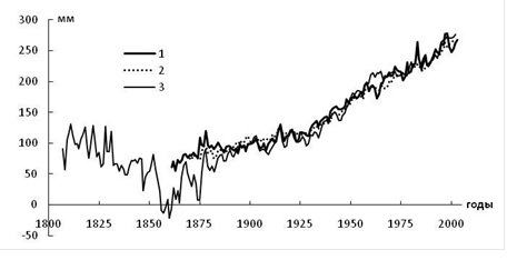
Fig. 1. Comparison of global sea level time series calculated by different authors. 1 – RSHU model [5], 2 – data of Church and White, 2006 [1], 3 – data of Jevrejeva et al. 2006 [6].
Average rate of GSL rise for the considered period is about 1.4 mm/year, and the trend describes 94% of dispersion of the initial row. Thus, the observed powerful linear trend is the main regularity of interannual fluctuations of global sea level. In the GSL main trend there are several distinct periods of various origin of level changes that have different local trends. It is a quite rapid growth of GSL in 1861-1877 (Tr = 2.0 mm/year), followed by the period of 1879-1923 when the level remained almost the same, i.e. there was a phase of nearly-standing level (Tr = 0.4 mm/year); after that up to the present it has been again rising rapidly (Tr = 2.0 mm/year). During the XX century the trend reached nearly 1.8 mm/year.
Note, that GSL calculated on our statistical model is fully compatible with the similar GSL reconstructions of other authors [1,6] based on data including over 1000 stations of global archive of sea level gauges PSMSL. The model certain advantage against the western analogs is that with the same level of accuracy it calculates GSL with a minimum of initial information, namely, data from only several stationary coastal stations.
We found that the trend formation in annual GSL can be considered in the form of a "random walk" statistical model [3]. The essence of the model is in the consecutive summation of intra-annual level increment values (DhМ), representing the stationary casual process developing in the form of a "red noise" model. The trend of this new row is completely identical to a trend of GSL average annual values, i.e. Tr(SDhМ) = Tr(hM). The physical sense of this result is that during the assessment of the contribution of different factors to GSL trend formation it is possible to use the equations of fresh-water budget of the ocean and the changes of water budget of the hydrosphere.
The study of the genesis of GSL interannual fluctuations is possible on the basis of two main approaches. From the equation of the water budget in the hydrosphere representing the system of interacting reservoirs consisting of the ocean, the atmosphere, the cryosphere and fresh waters of land, GSL changes can be presented in the form:
DhM = АМ–1(–DVC –DVL + DVster), (1)
where DhM – sea level intra-annual fluctuations; АМ – World Ocean area; DVC – fluctuations of cryosphere water mass; DVL – fluctuations of fresh water mass (land and ground waters), DVster – fluctuations of GSL steric component due to changes of ocean heat content. This is the equation used in foreign studies on assessment of contribution of various factors to GSL changes. Generalization of the obtained results is presented in the Assessment Reports of the Intergovernmental Panel on Climate Change (IPCC), and in the multi-author monograph [7].
Another approach developed in RSHU is the assessment of contribution of various factors performed with the equation of fresh-water budget of the World Ocean as a sum of eustatic and steric factors. Therefore, we have:
D hM = АМ –1(PWO + M + I – EWO + D Vster), (2)
where PWO – precipitation on the surface of the World Ocean (WO); M – land (surface and ground) flow to WO; I – ice flow to WO; EWO – evaporation from the surface of WO.
Foreign researchers use the method of trends, i.e. linear trends of “sea level forming” factors are calculated for various periods and then their sums are compared with the actual trend of GSL. It is clear, that the method of trends is adequate only for monotonous data rows and allows a quite approximate judgement of the contribution of separate factors because of the strong dependence on the trend value and the contribution of the trend coefficient of determination to dispersion of the initial process. It is known that for short rows the trend value depends on the row length, and the row length changes only on one value can cause the significant change of the trend value, up to the sign change.
III. results and discussion
Let’s consider the generalizing results of numerous studies on assessment of contribution of various factors to the GSL trend presented in IPCC reports. In the XX century (1910-1990) the total contribution of the “sea level forming” factors (with mountain glaciers) ranged from -0.8 to 2.2 mm/year with the average value of 0.7 mm/year (Table 1) [8]. If we exclude the thawing of mountain glaciers from total contribution the total value will decrease to 0.4 mm/year. It is obvious that IPCC experts make a principal mistake here, considering the thawing of mountain glaciers as a contribution to GSL changes. Thawing of mountain glaciers, which is indeed very essential, can give a direct contribution to GSL changes only from the glaciers located on islands in the Arctic Ocean, and perhaps partially from the territory of Alaska, and therefore their contribution to GSL rise does not exceed 0.1 mm/year. Mountain glaciers in Europe, Asia, Africa and South America can influence GSL only through the flow of river water to the ocean. Therefore, it is hardly necessary to consider their direct contribution to the GSL trend.
Because the actual rise of GSL according to observations was Tr = 1.5 mm/year, we have a huge residual error (imbalance) between the calculated and actual trend values in GSL, exceeding the contribution of any of the “sea level forming” factor.
Table 1. Contributions of various factors to GSL trend formation based on the IPCC Reports
|
GSL driving factors |
Trend values, mm/year |
|||
|
1910-1990 [8] |
1961-2003 [9] |
1993-2003 [9] |
1993-2010 [2] |
|
|
Thermal expansion |
0,51 ± 0,20 |
0,42 ± 0,12 |
1,6 ± 0,5 |
1,1 (0,8-1,4) |
|
Glaciers and icecaps |
0,30 ± 0,09 |
0,5 ± 0,18 |
0,77 ± 0,22 |
0,76 (0,39-1,13) |
|
Greenland Ice Sheet |
0,06 ± 0,05 |
0,05 ± 0,12 |
0,21 ± 0,07 |
0,33 (0,25-0,41)
|
|
Antarctic Ice Sheet |
-0,09 ± 0,10 |
0,14 ± 0,41 |
0,21 ± 0,35 |
0,27 (0,16-0,38)
|
|
Land waters |
-0,07 ± 0,78 |
- |
- |
0,38 (0,26-0,49) |
|
Total |
0,70 ± 0,82 |
1,1 ± 0,5 |
2,8 ± 0,7 |
2,8 (2,3-3,4) |
|
Observed sea level |
1,5 ± 0,50 |
1,8 ± 0,5 |
3,1 ± 0,7 |
3,2 (2,8-3,6) |
The same high residual errors are observed for other periods. For the period 1961-2003 the residual error without mountain glaciers makes 1.0 mm/year, and for 1993-2003 – 0.9 mm/year [9], for 1993-2010 – 1.2 mm/year [2], and on absolute value they exceed the contribution of any factor of GSL formation (Table 1). Highly doubtable is also the assessment of considerable reduction of surface and ground water reserves which contribution to GSL trend for 1993-2010 (based on data from [2]) was 0.38 mm/year exceeding the contribution of ice sheets of Antarctica and Greenland. This must by all means be manifested in the sharp growth of continental flow to the World Ocean. However, Russian scientists do not confirm this fact [10, 11]. Therefore, we can surely claim that the use of the equation of water mass budget in the hydrosphere for the GSL trend assessment by foreign researchers is hardly justified because it requires the knowledge of a large number of the different difficult to determine factors which accuracy in many cases even can not be checked.
In our opinion, to assess the role of different factors in GSL trend formation the equation (2) should be used with easier determined components than the components of the equation (1), and with the accuracy that is possible to check [12]. The study [4] presents the assessment of interannual variability of evaporation and rainfall, and their difference on the basis of CDAS reanalysis (Climate Data Assimilation System) for the period of global warming (1980-2006). The pronounced positive trend describing more than 50% of dispersion is characteristic of time series of rainfall and evaporation. The trend for rainfall over the World Ocean is Tr = 4.2 mm/year, and for evaporation Tr = 3.6 mm/year; respectively the trend in effective evaporation is negative. Thereof, during 1980-2005 there was a GSL rise at a rate of 0.6 mm/year corresponding to 217 km3/year. Correlation of series of evaporation and rainfall with global air temperature makes r = 0.82 and r = 0.80 respectively.
The RSHU studies of various “sea level forming” factors allowed to perform a comparison of the actual and calculated GSL trends for two periods (1980–2005 and 1993-2003) shown in Table 2. Here the calculated GSL trend was determined as a sum of trends of eustatic and steric components. It is easy to see that the residual error of calculations makes respectively 0.21 and 0.22 mm/year. It is more than three times lower than the IPCC estimates in case of excluding the contribution of mountain glaciers.
Table 2. Estimates of the contribution of various factors to GSL trend formation for 1980–2005 and 1993-2003 using the equation of fresh-water budget of the World Ocean, mm/year, based on data from [3]
|
Sources of GSL rise |
1980–2005 |
1993–2003 |
|
Steric sea level fluctuations Total flow from Solid flow from Input of land waters Vertical water exchange (rainfall minus evaporation) |
0,30 0,14 0,24 0,16 0,62 |
1,60 0,22 0,44 0,19 0,43 |
|
Total contribution of factors |
1,56 |
2,88 |
|
GSL rise based on observations |
1,79 |
3,10 |
|
Misbalance (residual error) |
0,23 |
0,22 |
A complex of methods of GSL longterm forecast was developed in RSHU for the first time: long-range forecast (century), short-range forecast (several decades) and for the current period (several years). Such division is explained, on one hand, by physical regularities of the sea level fluctuations and influence of various factors, and on the other hand – by practical needs of consumers. For long-range forecasting (for the end of the XXI century) the simple statistical GSL forecasting model [13] is offered. It is based on the use of the global air temperature (GAT) modelling with a complex of numerical models of ocean and atmosphere circulation (OACM). The comparison of global estimates of GAT anomalies and GSL values during 1960-2008 based on coastal observational data showed a well expressed linear dependence between them. This allowed to calculate a linear statistical model which describes 73% of GSL dispersion.
A probable range of GSL rise for the end of 2090-2099 [9] was calculated on the statistical model for the 6 main scenarios of climate change and with the probable range of temperature rise for the end of 2090-2099 set according to a complex of 16 climatic models. The comparison of predicted GSL data for the end of the XXI century on the statistical model and on the OACM complex showed almost full agreement (Table 3). The obvious advantage of the model is that it requires a minimum of initial information, providing at the same time the same level of accuracy as in the complex and expensive OACM. This means that in approximate predictive GSL calculations it is quite reasonable to exclude the use of OACM.
Table 3. Estimates of possible changes of global surface temperature and global sea level by the end of XXI century (2090-2099) as compared to the end of ХХ century (1980 – 1999)
|
Emission scenario |
Ensemble of 16 models of ocean and atmosphere circulation [9] |
Statistical model [13] |
|
|
Probable range of temperature rise by 2090-2099, оС |
Probable range of GSL rise by 2090–2099, m |
Probable range of GSL rise by 2090–2099, m |
|
|
Scenario B1 |
1,1 – 2,9 |
0,18 – 0,38 |
0,12 – 0,31 |
|
Scenario A1T |
1,4 – 3,8 |
0,30 – 0,45 |
0,15 – 0,41 |
|
Scenario B2 |
1,4 – 3,8 |
0,20 – 0,43 |
0,15 – 0,41 |
|
Scenario A1B |
1,7 – 4,4 |
0,21 – 0,48 |
0,18 – 0,47 |
|
Scenario A2 |
2,0 – 5,4 |
0,23 – 0,51 |
0,21 - 0,58 |
|
Scenario A1FI |
2,4 – 6,4 |
0,26 – 0,59 |
0,26 – 0,68 |
The physical and statistical model of interannual fluctuations of global sea level is developed and presented in order to predict the long-term changes for two decades [14] which does not have analogs in foreign studies. It is based on the formulated concept that GAT changes are the most important defining factor of GSL variations. It was experimentally shown that there is a long delay (20 and 30 years) of GSL fluctuations in relation to GAT changes. It allows to use the procedure of the shift step-wise multiple regression for determination of optimum models of GSL fluctuations depending on air temperature values set at the nodes of the grid area over the ocean. A complete complex of step-wise models was calculated on the dependent series (1901-1999) for shifts from τ = 0 to τ = 33 years by the method of inclusion of variables up to 15 predictors, so that the total number of models was over 500. Their analysis allowed to set the shift of τ = 21 years when the GAT influence on GSL fluctuations is manifested at the maximum level. As a result it was possible to calculate the prognostic estimates of GSL up until 2028 (Figure 2). The trend value for the specified period is Tr = 3.0 mm/year that satisfactorily corresponds to the altimetry GSL trend value (2.9-3.0 mm/year) for the beginning of XXI century. The adequacy of obtained results was confirmed by the similar physical and statistical models constructed for GSL time series taken from studies [1, 6].
.jpg)
Fig. 2. Predicted GSL for 2000-2028 calculated on the statistical model for different amount of parameters from m=1 to m=19 [14]. Solid line – averaged curve for 19 GSL values for each year.
IV. conclusion
As a conclusion and summing up the results we can say that the Russian leader in the study and forecasting of global sea level fluctuations can be considered Russian State Hydrometeorological University. This direction owing to the huge practical value within many decades will remain the most important problem of modern hydrometeorology
1. Church J.A., White N.J. A 20th century acceleration in global sea-level rise // Geophysical Res. Letters. 2006, V. 33. N 1. L01602.
2. IPCC. Climate Change 2013: The Physical Science Basis. Contribution of Working Group to the Fifth Assessment Report of the Intergovernmental Panel on Climate Change / Eds. Stocker T.F. at al. Cambridge (UK); N. Y.: Cambridge University Press, 2013.1535 pp.
3. Malinin V.N. Global sea level: present and future. St.Petersburg: RSHU, 2012. 260 p.
4. Malinin V.N. Global water budget. - Lambert Academic Publishing, 2011, 158 p.
5. Malinin V.N., Gordeeva S.M., Shevchyk O.I. Variability of global sea level in last 140 years. Uchenye zapiski RGGMU. 2007. Vol. 4. p.125-132.
6. Jevrejeva S., Grinsted A., Moore J.C., Holgate S. Nonlinear trends and multiyear cycles in sea level records // J. Geophys. Res. 2006, V. 111. N C9. C09012.
7. Understanding Sea-level Rise and Variability // Eds. John A. Church, Philip L. Woodworth, Thorkild Aarup, W. Stanley Wilson.- Wiley-Blackwell, 2010. 456 p. ISBN: 978-1-4443-3451-7.
8. IPCC. Climate Change 2001: The Scientific Basis. Contribution of Working Group I to the Third Assessment Report of the Intergovernmental Panel on Climate Change / Eds. Houghton, J.T. et al.- Cambridge; New York, Cambridge university press. 2001. 881 p.
9. IPCC. Climate Change 2007: The Physical Science Basis. Intergovernmental Panel on Climate Change Fourth Assessment Report Climate Change 2007 / Eds. Bernstein L. et al.- Cambridge; New York, Cambridge University Press. 2007. 940 r.
10. Babkin V.I., Klige R.K. River flow to the World Ocean // Uchenie zapiski RGGMU. 2009. Vol. 13, p. 17-20.
11. Dobrovolskiy S.G. Global changes of river flow. - Moscow: GEOS, 2011, 660 p.
12. Malinin V.N. Water exchange in the system ocean-atmosphere. - Leningrad: Hydrometeoizdat, 1994, 197 p.
13. Malinina U.V. To the assessment of possible damage from expected sea level rise in XXI // Uchenye zapiski RGGMY. 2010. №14. p.162-176.
14. Malinin V.N., Shevchyk O.I. On possible global sea level changes in future decades // Obshchestvo. Sreda. Razvitie, 2009, №2, p.172-180.